


Pandas 組操作

By “group by” we are referring to a process involving one or more of the following steps:
- Splitting the data into groups based on some criteria.
- Applying a function to each group independently.
- Combining the results into a data structure.
Out of these, the split step is the most straightforward. In fact, in many situations we may wish to split the data set into groups and do something with those groups. In the apply step, we might wish to do one of the following:
Aggregation: compute a summary statistic (or statistics) for each group. Some examples:
- Compute group sums or means.
- Compute group sizes / counts.
Transformation: perform some group-specific computations and return a like-indexed object. Some examples:
- Standardize data (zscore) within a group.
- Filling NAs within groups with a value derived from each group.
Filtration: discard some groups, according to a group-wise computation that evaluates True or False. Some examples:
- Discard data that belongs to groups with only a few members.
- Filter out data based on the group sum or mean.
Some combination of the above: GroupBy will examine the results of the apply step and try to return a sensibly combined result if it doesn’t fit into either of the above two categories.
Since the set of object instance methods on pandas data structures are generally rich and expressive, we often simply want to invoke, say, a DataFrame function on each group. The name GroupBy should be quite familiar to those who have used a SQL-based tool (or itertools), in which you can write code like:
SELECT Column1, Column2, mean(Column3), sum(Column4)
FROM SomeTable
GROUP BY Column1, Column2
We aim to make operations like this natural and easy to express using pandas. We’ll address each area of GroupBy functionality then provide some non-trivial examples / use cases.
See the cookbook for some advanced strategies.
#Splitting an object into groups
pandas objects can be split on any of their axes. The abstract definition of grouping is to provide a mapping of labels to group names. To create a GroupBy object (more on what the GroupBy object is later), you may do the following:
In [1]: df = pd.DataFrame([('bird', 'Falconiformes', 389.0),
   ...:                    ('bird', 'Psittaciformes', 24.0),
   ...:                    ('mammal', 'Carnivora', 80.2),
   ...:                    ('mammal', 'Primates', np.nan),
   ...:                    ('mammal', 'Carnivora', 58)],
   ...:                   index=['falcon', 'parrot', 'lion', 'monkey', 'leopard'],
   ...:                   columns=('class', 'order', 'max_speed'))
   ...:

In [2]: df
Out[2]:
          class           order  max_speed
falcon     bird   Falconiformes      389.0
parrot     bird  Psittaciformes       24.0
lion     mammal       Carnivora       80.2
monkey   mammal        Primates        NaN
leopard  mammal       Carnivora       58.0

# default is axis=0
In [3]: grouped = df.groupby('class')

In [4]: grouped = df.groupby('order', axis='columns')

In [5]: grouped = df.groupby(['class', 'order'])
The mapping can be specified many different ways:
- A Python function, to be called on each of the axis labels.
- A list or NumPy array of the same length as the selected axis.
- A dict or
Series, providing alabel -> group namemapping. - For
DataFrameobjects, a string indicating a column to be used to group. Of coursedf.groupby('A')is just syntactic sugar fordf.groupby(df['A']), but it makes life simpler. - For
DataFrameobjects, a string indicating an index level to be used to group. - A list of any of the above things.
Collectively we refer to the grouping objects as the keys. For example, consider the following DataFrame:
Note
A string passed to groupby may refer to either a column or an index level. If a string matches both a column name and an index level name, a ValueError will be raised.
In [6]: df = pd.DataFrame({'A': ['foo', 'bar', 'foo', 'bar',
   ...:                          'foo', 'bar', 'foo', 'foo'],
   ...:                    'B': ['one', 'one', 'two', 'three',
   ...:                          'two', 'two', 'one', 'three'],
   ...:                    'C': np.random.randn(8),
   ...:                    'D': np.random.randn(8)})
   ...:

In [7]: df
Out[7]:
     A      B         C         D
0  foo    one  0.469112 -0.861849
1  bar    one -0.282863 -2.104569
2  foo    two -1.509059 -0.494929
3  bar  three -1.135632  1.071804
4  foo    two  1.212112  0.721555
5  bar    two -0.173215 -0.706771
6  foo    one  0.119209 -1.039575
7  foo  three -1.044236  0.271860
On a DataFrame, we obtain a GroupBy object by calling groupby()We could naturally group by either the A or B columns, or both:
In [8]: grouped = df.groupby('A')

In [9]: grouped = df.groupby(['A', 'B'])
New in version 0.24.
If we also have a MultiIndex on columns A and B, we can group by all but the specified columns
In [10]: df2 = df.set_index(['A', 'B'])

In [11]: grouped = df2.groupby(level=df2.index.names.difference(['B']))

In [12]: grouped.sum()
Out[12]:
            C         D
A
bar -1.591710 -1.739537
foo -0.752861 -1.402938
These will split the DataFrame on its index (rows). We could also split by the columns:
In [13]: def get_letter_type(letter):
   ....:     if letter.lower() in 'aeiou':
   ....:         return 'vowel'
   ....:     else:
   ....:         return 'consonant'
   ....:

In [14]: grouped = df.groupby(get_letter_type, axis=1)
pandas Indexobjects support duplicate values. If a non-unique index is used as the group key in a groupby operation, all values for the same index value will be considered to be in one group and thus the output of aggregation functions will only contain unique index values:
In [15]: lst = [1, 2, 3, 1, 2, 3]

In [16]: s = pd.Series([1, 2, 3, 10, 20, 30], lst)

In [17]: grouped = s.groupby(level=0)

In [18]: grouped.first()
Out[18]:
1    1
2    2
3    3
dtype: int64

In [19]: grouped.last()
Out[19]:
1    10
2    20
3    30
dtype: int64

In [20]: grouped.sum()
Out[20]:
1    11
2    22
3    33
dtype: int64
Note that no splitting occurs until it’s needed. Creating the GroupBy object only verifies that you’ve passed a valid mapping.
Note
Many kinds of complicated data manipulations can be expressed in terms of GroupBy operations (though can’t be guaranteed to be the most efficient). You can get quite creative with the label mapping functions.
#GroupBy sorting
By default the group keys are sorted during the groupby operation. You may however pass sort=False for potential speedups:
In [21]: df2 = pd.DataFrame({'X': ['B', 'B', 'A', 'A'], 'Y': [1, 2, 3, 4]})

In [22]: df2.groupby(['X']).sum()
Out[22]:
   Y
X
A  7
B  3

In [23]: df2.groupby(['X'], sort=False).sum()
Out[23]:
   Y
X
B  3
A  7
Note that groupby will preserve the order in which observations are sorted within each group. For example, the groups created by groupby() below are in the order they appeared in the original DataFrame:
In [24]: df3 = pd.DataFrame({'X': ['A', 'B', 'A', 'B'], 'Y': [1, 4, 3, 2]})

In [25]: df3.groupby(['X']).get_group('A')
Out[25]:
   X  Y
0  A  1
2  A  3

In [26]: df3.groupby(['X']).get_group('B')
Out[26]:
   X  Y
1  B  4
3  B  2
#GroupBy object attributes
The groups attribute is a dict whose keys are the computed unique groups and corresponding values being the axis labels belonging to each group. In the above example we have:
In [27]: df.groupby('A').groups
Out[27]:
{'bar': Int64Index([1, 3, 5], dtype='int64'),
 'foo': Int64Index([0, 2, 4, 6, 7], dtype='int64')}

In [28]: df.groupby(get_letter_type, axis=1).groups
Out[28]:
{'consonant': Index(['B', 'C', 'D'], dtype='object'),
 'vowel': Index(['A'], dtype='object')}
Calling the standard Python len function on the GroupBy object just returns the length of the groups dict, so it is largely just a convenience:
In [29]: grouped = df.groupby(['A', 'B'])

In [30]: grouped.groups
Out[30]:
{('bar', 'one'): Int64Index([1], dtype='int64'),
 ('bar', 'three'): Int64Index([3], dtype='int64'),
 ('bar', 'two'): Int64Index([5], dtype='int64'),
 ('foo', 'one'): Int64Index([0, 6], dtype='int64'),
 ('foo', 'three'): Int64Index([7], dtype='int64'),
 ('foo', 'two'): Int64Index([2, 4], dtype='int64')}

In [31]: len(grouped)
Out[31]: 6
GroupBy will tab complete column names (and other attributes):
In [32]: df
Out[32]:
               height      weight  gender
2000-01-01  42.849980  157.500553    male
2000-01-02  49.607315  177.340407    male
2000-01-03  56.293531  171.524640    male
2000-01-04  48.421077  144.251986  female
2000-01-05  46.556882  152.526206    male
2000-01-06  68.448851  168.272968  female
2000-01-07  70.757698  136.431469    male
2000-01-08  58.909500  176.499753  female
2000-01-09  76.435631  174.094104  female
2000-01-10  45.306120  177.540920    male

In [33]: gb = df.groupby('gender')
In [34]: gb.<TAB>  # noqa: E225, E999
gb.agg        gb.boxplot    gb.cummin     gb.describe   gb.filter     gb.get_group  gb.height     gb.last       gb.median     gb.ngroups    gb.plot       gb.rank       gb.std        gb.transform
gb.aggregate  gb.count      gb.cumprod    gb.dtype      gb.first      gb.groups     gb.hist       gb.max        gb.min        gb.nth        gb.prod       gb.resample   gb.sum        gb.var
gb.apply      gb.cummax     gb.cumsum     gb.fillna     gb.gender     gb.head       gb.indices    gb.mean       gb.name       gb.ohlc       gb.quantile   gb.size       gb.tail       gb.weight
#GroupBy with MultiIndex
With hierarchically-indexed data, it’s quite natural to group by one of the levels of the hierarchy.
Let’s create a Series with a two-level MultiIndex.
In [35]: arrays = [['bar', 'bar', 'baz', 'baz', 'foo', 'foo', 'qux', 'qux'],
   ....:           ['one', 'two', 'one', 'two', 'one', 'two', 'one', 'two']]
   ....:

In [36]: index = pd.MultiIndex.from_arrays(arrays, names=['first', 'second'])

In [37]: s = pd.Series(np.random.randn(8), index=index)

In [38]: s
Out[38]:
first  second
bar    one      -0.919854
       two      -0.042379
baz    one       1.247642
       two      -0.009920
foo    one       0.290213
       two       0.495767
qux    one       0.362949
       two       1.548106
dtype: float64
We can then group by one of the levels in s.
In [39]: grouped = s.groupby(level=0)

In [40]: grouped.sum()
Out[40]:
first
bar   -0.962232
baz    1.237723
foo    0.785980
qux    1.911055
dtype: float64
If the MultiIndex has names specified, these can be passed instead of the level number:
In [41]: s.groupby(level='second').sum()
Out[41]:
second
one    0.980950
two    1.991575
dtype: float64
The aggregation functions such as sum will take the level parameter directly. Additionally, the resulting index will be named according to the chosen level:
In [42]: s.sum(level='second')
Out[42]:
second
one    0.980950
two    1.991575
dtype: float64
Grouping with multiple levels is supported.
In [43]: s
Out[43]:
first  second  third
bar    doo     one     -1.131345
               two     -0.089329
baz    bee     one      0.337863
               two     -0.945867
foo    bop     one     -0.932132
               two      1.956030
qux    bop     one      0.017587
               two     -0.016692
dtype: float64

In [44]: s.groupby(level=['first', 'second']).sum()
Out[44]:
first  second
bar    doo      -1.220674
baz    bee      -0.608004
foo    bop       1.023898
qux    bop       0.000895
dtype: float64
New in version 0.20.
Index level names may be supplied as keys.
In [45]: s.groupby(['first', 'second']).sum()
Out[45]:
first  second
bar    doo      -1.220674
baz    bee      -0.608004
foo    bop       1.023898
qux    bop       0.000895
dtype: float64
More on the sum function and aggregation later.
#Grouping DataFrame with Index levels and columns
A DataFrame may be grouped by a combination of columns and index levels by specifying the column names as strings and the index levels as pd.Grouper objects.
In [46]: arrays = [['bar', 'bar', 'baz', 'baz', 'foo', 'foo', 'qux', 'qux'],
   ....:           ['one', 'two', 'one', 'two', 'one', 'two', 'one', 'two']]
   ....:

In [47]: index = pd.MultiIndex.from_arrays(arrays, names=['first', 'second'])

In [48]: df = pd.DataFrame({'A': [1, 1, 1, 1, 2, 2, 3, 3],
   ....:                    'B': np.arange(8)},
   ....:                   index=index)
   ....:

In [49]: df
Out[49]:
              A  B
first second
bar   one     1  0
      two     1  1
baz   one     1  2
      two     1  3
foo   one     2  4
      two     2  5
qux   one     3  6
      two     3  7
The following example groups df by the second index level and the A column.
In [50]: df.groupby([pd.Grouper(level=1), 'A']).sum()
Out[50]:
          B
second A
one    1  2
       2  4
       3  6
two    1  4
       2  5
       3  7
Index levels may also be specified by name.
In [51]: df.groupby([pd.Grouper(level='second'), 'A']).sum()
Out[51]:
          B
second A
one    1  2
       2  4
       3  6
two    1  4
       2  5
       3  7
New in version 0.20.
Index level names may be specified as keys directly to groupby.
In [52]: df.groupby(['second', 'A']).sum()
Out[52]:
          B
second A
one    1  2
       2  4
       3  6
two    1  4
       2  5
       3  7
#DataFrame column selection in GroupBy
Once you have created the GroupBy object from a DataFrame, you might want to do something different for each of the columns. Thus, using [] similar to getting a column from a DataFrame, you can do:
In [53]: grouped = df.groupby(['A'])

In [54]: grouped_C = grouped['C']

In [55]: grouped_D = grouped['D']
This is mainly syntactic sugar for the alternative and much more verbose:
In [56]: df['C'].groupby(df['A'])
Out[56]: <pandas.core.groupby.generic.SeriesGroupBy object at 0x7f65f21ac518>
Additionally this method avoids recomputing the internal grouping information derived from the passed key.
#Iterating through groups
With the GroupBy object in hand, iterating through the grouped data is very natural and functions similarly to itertools.groupby()
In [57]: grouped = df.groupby('A')

In [58]: for name, group in grouped:
   ....:     print(name)
   ....:     print(group)
   ....:
bar
     A      B         C         D
1  bar    one  0.254161  1.511763
3  bar  three  0.215897 -0.990582
5  bar    two -0.077118  1.211526
foo
     A      B         C         D
0  foo    one -0.575247  1.346061
2  foo    two -1.143704  1.627081
4  foo    two  1.193555 -0.441652
6  foo    one -0.408530  0.268520
7  foo  three -0.862495  0.024580
In the case of grouping by multiple keys, the group name will be a tuple:
In [59]: for name, group in df.groupby(['A', 'B']):
   ....:     print(name)
   ....:     print(group)
   ....:
('bar', 'one')
     A    B         C         D
1  bar  one  0.254161  1.511763
('bar', 'three')
     A      B         C         D
3  bar  three  0.215897 -0.990582
('bar', 'two')
     A    B         C         D
5  bar  two -0.077118  1.211526
('foo', 'one')
     A    B         C         D
0  foo  one -0.575247  1.346061
6  foo  one -0.408530  0.268520
('foo', 'three')
     A      B         C        D
7  foo  three -0.862495  0.02458
('foo', 'two')
     A    B         C         D
2  foo  two -1.143704  1.627081
4  foo  two  1.193555 -0.441652
See Iterating through groups.
#Selecting a group
A single group can be selected using get_group():
In [60]: grouped.get_group('bar')
Out[60]:
     A      B         C         D
1  bar    one  0.254161  1.511763
3  bar  three  0.215897 -0.990582
5  bar    two -0.077118  1.211526
Or for an object grouped on multiple columns:
In [61]: df.groupby(['A', 'B']).get_group(('bar', 'one'))
Out[61]:
     A    B         C         D
1  bar  one  0.254161  1.511763
#Aggregation
Once the GroupBy object has been created, several methods are available to perform a computation on the grouped data. These operations are similar to the aggregating API window functions API, and resample API.
An obvious one is aggregation via the aggregate() or equivalently agg() method:
In [62]: grouped = df.groupby('A')

In [63]: grouped.aggregate(np.sum)
Out[63]:
            C         D
A
bar  0.392940  1.732707
foo -1.796421  2.824590

In [64]: grouped = df.groupby(['A', 'B'])

In [65]: grouped.aggregate(np.sum)
Out[65]:
                  C         D
A   B
bar one    0.254161  1.511763
    three  0.215897 -0.990582
    two   -0.077118  1.211526
foo one   -0.983776  1.614581
    three -0.862495  0.024580
    two    0.049851  1.185429
As you can see, the result of the aggregation will have the group names as the new index along the grouped axis. In the case of multiple keys, the result is a MultiIndex by default, though this can be changed by using the as_index option:
In [66]: grouped = df.groupby(['A', 'B'], as_index=False)

In [67]: grouped.aggregate(np.sum)
Out[67]:
     A      B         C         D
0  bar    one  0.254161  1.511763
1  bar  three  0.215897 -0.990582
2  bar    two -0.077118  1.211526
3  foo    one -0.983776  1.614581
4  foo  three -0.862495  0.024580
5  foo    two  0.049851  1.185429

In [68]: df.groupby('A', as_index=False).sum()
Out[68]:
     A         C         D
0  bar  0.392940  1.732707
1  foo -1.796421  2.824590
Note that you could use the reset_index DataFrame function to achieve the same result as the column names are stored in the resulting MultiIndex:
In [69]: df.groupby(['A', 'B']).sum().reset_index()
Out[69]:
     A      B         C         D
0  bar    one  0.254161  1.511763
1  bar  three  0.215897 -0.990582
2  bar    two -0.077118  1.211526
3  foo    one -0.983776  1.614581
4  foo  three -0.862495  0.024580
5  foo    two  0.049851  1.185429
Another simple aggregation example is to compute the size of each group. This is included in GroupBy as the size method. It returns a Series whose index are the group names and whose values are the sizes of each group.
In [70]: grouped.size()
Out[70]:
A    B
bar  one      1
     three    1
     two      1
foo  one      2
     three    1
     two      2
dtype: int64
In [71]: grouped.describe()
Out[71]:
      C                                                                           D
  count      mean       std       min       25%       50%       75%       max count      mean       std       min       25%       50%       75%       max
0   1.0  0.254161       NaN  0.254161  0.254161  0.254161  0.254161  0.254161   1.0  1.511763       NaN  1.511763  1.511763  1.511763  1.511763  1.511763
1   1.0  0.215897       NaN  0.215897  0.215897  0.215897  0.215897  0.215897   1.0 -0.990582       NaN -0.990582 -0.990582 -0.990582 -0.990582 -0.990582
2   1.0 -0.077118       NaN -0.077118 -0.077118 -0.077118 -0.077118 -0.077118   1.0  1.211526       NaN  1.211526  1.211526  1.211526  1.211526  1.211526
3   2.0 -0.491888  0.117887 -0.575247 -0.533567 -0.491888 -0.450209 -0.408530   2.0  0.807291  0.761937  0.268520  0.537905  0.807291  1.076676  1.346061
4   1.0 -0.862495       NaN -0.862495 -0.862495 -0.862495 -0.862495 -0.862495   1.0  0.024580       NaN  0.024580  0.024580  0.024580  0.024580  0.024580
5   2.0  0.024925  1.652692 -1.143704 -0.559389  0.024925  0.609240  1.193555   2.0  0.592714  1.462816 -0.441652  0.075531  0.592714  1.109898  1.627081
Note
Aggregation functions will not return the groups that you are aggregating over if they are named columns, when as_index=True, the default. The grouped columns will be the indices of the returned object.
Passing as_index=False will return the groups that you are aggregating over, if they are named columns.
Aggregating functions are the ones that reduce the dimension of the returned objects. Some common aggregating functions are tabulated below:
| Function | Description |
|---|---|
| mean() | Compute mean of groups |
| sum() | Compute sum of group values |
| size() | Compute group sizes |
| count() | Compute count of group |
| std() | Standard deviation of groups |
| var() | Compute variance of groups |
| sem() | Standard error of the mean of groups |
| describe() | Generates descriptive statistics |
| first() | Compute first of group values |
| last() | Compute last of group values |
| nth() | Take nth value, or a subset if n is a list |
| min() | Compute min of group values |
| max() | Compute max of group values |
The aggregating functions above will exclude NA values. Any function which reduces a Series to a scalar value is an aggregation function and will work, a trivial example is df.groupby('A').agg(lambda ser: 1). Note that nth() can act as a reducer or a filter, see here.
#Applying multiple functions at once
With grouped Series you can also pass a list or dict of functions to do aggregation with, outputting a DataFrame:
In [72]: grouped = df.groupby('A')

In [73]: grouped['C'].agg([np.sum, np.mean, np.std])
Out[73]:
          sum      mean       std
A
bar  0.392940  0.130980  0.181231
foo -1.796421 -0.359284  0.912265
On a grouped DataFrame, you can pass a list of functions to apply to each column, which produces an aggregated result with a hierarchical index:
In [74]: grouped.agg([np.sum, np.mean, np.std])
Out[74]:
            C                             D
          sum      mean       std       sum      mean       std
A
bar  0.392940  0.130980  0.181231  1.732707  0.577569  1.366330
foo -1.796421 -0.359284  0.912265  2.824590  0.564918  0.884785
The resulting aggregations are named for the functions themselves. If you need to rename, then you can add in a chained operation for a Series like this:
In [75]: (grouped['C'].agg([np.sum, np.mean, np.std])
   ....:              .rename(columns={'sum': 'foo',
   ....:                               'mean': 'bar',
   ....:                               'std': 'baz'}))
   ....:
Out[75]:
          foo       bar       baz
A
bar  0.392940  0.130980  0.181231
foo -1.796421 -0.359284  0.912265
For a grouped DataFrame, you can rename in a similar manner:
In [76]: (grouped.agg([np.sum, np.mean, np.std])
   ....:         .rename(columns={'sum': 'foo',
   ....:                          'mean': 'bar',
   ....:                          'std': 'baz'}))
   ....:
Out[76]:
            C                             D
          foo       bar       baz       foo       bar       baz
A
bar  0.392940  0.130980  0.181231  1.732707  0.577569  1.366330
foo -1.796421 -0.359284  0.912265  2.824590  0.564918  0.884785
Note
In general, the output column names should be unique. You can’t apply the same function (or two functions with the same name) to the same column.
In [77]: grouped['C'].agg(['sum', 'sum'])
---------------------------------------------------------------------------
SpecificationError                        Traceback (most recent call last)
<ipython-input-77-7be02859f395> in <module>
----> 1 grouped['C'].agg(['sum', 'sum'])

/pandas/pandas/core/groupby/generic.py in aggregate(self, func_or_funcs, *args, **kwargs)
    849             # but not the class list / tuple itself.
    850             func_or_funcs = _maybe_mangle_lambdas(func_or_funcs)
--> 851             ret = self._aggregate_multiple_funcs(func_or_funcs, (_level or 0) + 1)
    852             if relabeling:
    853                 ret.columns = columns

/pandas/pandas/core/groupby/generic.py in _aggregate_multiple_funcs(self, arg, _level)
    919                 raise SpecificationError(
    920                     "Function names must be unique, found multiple named "
--> 921                     "{}".format(name)
    922                 )
    923

SpecificationError: Function names must be unique, found multiple named sum
Pandas does allow you to provide multiple lambdas. In this case, pandas will mangle the name of the (nameless) lambda functions, appending _ to each subsequent lambda.
In [78]: grouped['C'].agg([lambda x: x.max() - x.min(),
   ....:                   lambda x: x.median() - x.mean()])
   ....:
Out[78]:
     <lambda_0>  <lambda_1>
A
bar    0.331279    0.084917
foo    2.337259   -0.215962
#Named aggregation
New in version 0.25.0.
To support column-specific aggregation with control over the output column names, pandas accepts the special syntax in GroupBy.agg(), known as “named aggregation”, where
- The keywords are the output column names
- The values are tuples whose first element is the column to select and the second element is the aggregation to apply to that column. Pandas provides the
pandas.NamedAggnamedtuple with the fields['column', 'aggfunc']to make it clearer what the arguments are. As usual, the aggregation can be a callable or a string alias.
In [79]: animals = pd.DataFrame({'kind': ['cat', 'dog', 'cat', 'dog'],
   ....:                         'height': [9.1, 6.0, 9.5, 34.0],
   ....:                         'weight': [7.9, 7.5, 9.9, 198.0]})
   ....:

In [80]: animals
Out[80]:
  kind  height  weight
0  cat     9.1     7.9
1  dog     6.0     7.5
2  cat     9.5     9.9
3  dog    34.0   198.0

In [81]: animals.groupby("kind").agg(
   ....:     min_height=pd.NamedAgg(column='height', aggfunc='min'),
   ....:     max_height=pd.NamedAgg(column='height', aggfunc='max'),
   ....:     average_weight=pd.NamedAgg(column='weight', aggfunc=np.mean),
   ....: )
   ....:
Out[81]:
      min_height  max_height  average_weight
kind
cat          9.1         9.5            8.90
dog          6.0        34.0          102.75
pandas.NamedAgg is just a namedtuple. Plain tuples are allowed as well.
In [82]: animals.groupby("kind").agg(
   ....:     min_height=('height', 'min'),
   ....:     max_height=('height', 'max'),
   ....:     average_weight=('weight', np.mean),
   ....: )
   ....:
Out[82]:
      min_height  max_height  average_weight
kind
cat          9.1         9.5            8.90
dog          6.0        34.0          102.75
If your desired output column names are not valid python keywords, construct a dictionary and unpack the keyword arguments
In [83]: animals.groupby("kind").agg(**{
   ....:     'total weight': pd.NamedAgg(column='weight', aggfunc=sum),
   ....: })
   ....:
Out[83]:
      total weight
kind
cat           17.8
dog          205.5
Additional keyword arguments are not passed through to the aggregation functions. Only pairs of (column, aggfunc) should be passed as **kwargs. If your aggregation functions requires additional arguments, partially apply them with functools.partial().
Note
For Python 3.5 and earlier, the order of **kwargs in a functions was not preserved. This means that the output column ordering would not be consistent. To ensure consistent ordering, the keys (and so output columns) will always be sorted for Python 3.5.
Named aggregation is also valid for Series groupby aggregations. In this case there’s no column selection, so the values are just the functions.
In [84]: animals.groupby("kind").height.agg(
   ....:     min_height='min',
   ....:     max_height='max',
   ....: )
   ....:
Out[84]:
      min_height  max_height
kind
cat          9.1         9.5
dog          6.0        34.0
#Applying different functions to DataFrame columns
By passing a dict to aggregate you can apply a different aggregation to the columns of a DataFrame:
In [85]: grouped.agg({'C': np.sum,
   ....:              'D': lambda x: np.std(x, ddof=1)})
   ....:
Out[85]:
            C         D
A
bar  0.392940  1.366330
foo -1.796421  0.884785
The function names can also be strings. In order for a string to be valid it must be either implemented on GroupBy or available via dispatching:
In [86]: grouped.agg({'C': 'sum', 'D': 'std'})
Out[86]:
            C         D
A
bar  0.392940  1.366330
foo -1.796421  0.884785
#Cython-optimized aggregation functions
Some common aggregations, currently only sum, mean, std, and sem, have optimized Cython implementations:
In [87]: df.groupby('A').sum()
Out[87]:
            C         D
A
bar  0.392940  1.732707
foo -1.796421  2.824590

In [88]: df.groupby(['A', 'B']).mean()
Out[88]:
                  C         D
A   B
bar one    0.254161  1.511763
    three  0.215897 -0.990582
    two   -0.077118  1.211526
foo one   -0.491888  0.807291
    three -0.862495  0.024580
    two    0.024925  0.592714
Of course sum and mean are implemented on pandas objects, so the above code would work even without the special versions via dispatching (see below).
#Transformation
The transform method returns an object that is indexed the same (same size) as the one being grouped. The transform function must:
- Return a result that is either the same size as the group chunk or broadcastable to the size of the group chunk (e.g., a scalar,
grouped.transform(lambda x: x.iloc[-1])). - Operate column-by-column on the group chunk. The transform is applied to the first group chunk using chunk.apply.
- Not perform in-place operations on the group chunk. Group chunks should be treated as immutable, and changes to a group chunk may produce unexpected results. For example, when using
fillna,inplacemust beFalse(grouped.transform(lambda x: x.fillna(inplace=False))). - (Optionally) operates on the entire group chunk. If this is supported, a fast path is used starting from the second chunk.
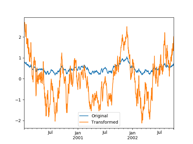
For example, suppose we wished to standardize the data within each group:
In [89]: index = pd.date_range('10/1/1999', periods=1100)

In [90]: ts = pd.Series(np.random.normal(0.5, 2, 1100), index)

In [91]: ts = ts.rolling(window=100, min_periods=100).mean().dropna()

In [92]: ts.head()
Out[92]:
2000-01-08    0.779333
2000-01-09    0.778852
2000-01-10    0.786476
2000-01-11    0.782797
2000-01-12    0.798110
Freq: D, dtype: float64

In [93]: ts.tail()
Out[93]:
2002-09-30    0.660294
2002-10-01    0.631095
2002-10-02    0.673601
2002-10-03    0.709213
2002-10-04    0.719369
Freq: D, dtype: float64

In [94]: transformed = (ts.groupby(lambda x: x.year)
   ....:                  .transform(lambda x: (x - x.mean()) / x.std()))
   ....:
We would expect the result to now have mean 0 and standard deviation 1 within each group, which we can easily check:
# Original Data
In [95]: grouped = ts.groupby(lambda x: x.year)

In [96]: grouped.mean()
Out[96]:
2000    0.442441
2001    0.526246
2002    0.459365
dtype: float64

In [97]: grouped.std()
Out[97]:
2000    0.131752
2001    0.210945
2002    0.128753
dtype: float64

# Transformed Data
In [98]: grouped_trans = transformed.groupby(lambda x: x.year)

In [99]: grouped_trans.mean()
Out[99]:
2000    1.168208e-15
2001    1.454544e-15
2002    1.726657e-15
dtype: float64

In [100]: grouped_trans.std()
Out[100]:
2000    1.0
2001    1.0
2002    1.0
dtype: float64
We can also visually compare the original and transformed data sets.
In [101]: compare = pd.DataFrame({'Original': ts, 'Transformed': transformed})

In [102]: compare.plot()
Out[102]: <matplotlib.axes._subplots.AxesSubplot at 0x7f65f731cba8>
Transformation functions that have lower dimension outputs are broadcast to match the shape of the input array.
In [103]: ts.groupby(lambda x: x.year).transform(lambda x: x.max() - x.min())
Out[103]:
2000-01-08    0.623893
2000-01-09    0.623893
2000-01-10    0.623893
2000-01-11    0.623893
2000-01-12    0.623893
                ...
2002-09-30    0.558275
2002-10-01    0.558275
2002-10-02    0.558275
2002-10-03    0.558275
2002-10-04    0.558275
Freq: D, Length: 1001, dtype: float64
Alternatively, the built-in methods could be used to produce the same outputs.
In [104]: max = ts.groupby(lambda x: x.year).transform('max')

In [105]: min = ts.groupby(lambda x: x.year).transform('min')

In [106]: max - min
Out[106]:
2000-01-08    0.623893
2000-01-09    0.623893
2000-01-10    0.623893
2000-01-11    0.623893
2000-01-12    0.623893
                ...
2002-09-30    0.558275
2002-10-01    0.558275
2002-10-02    0.558275
2002-10-03    0.558275
2002-10-04    0.558275
Freq: D, Length: 1001, dtype: float64
Another common data transform is to replace missing data with the group mean.
In [107]: data_df
Out[107]:
            A         B         C
0    1.539708 -1.166480  0.533026
1    1.302092 -0.505754       NaN
2   -0.371983  1.104803 -0.651520
3   -1.309622  1.118697 -1.161657
4   -1.924296  0.396437  0.812436
..        ...       ...       ...
995 -0.093110  0.683847 -0.774753
996 -0.185043  1.438572       NaN
997 -0.394469 -0.642343  0.011374
998 -1.174126  1.857148       NaN
999  0.234564  0.517098  0.393534

[1000 rows x 3 columns]

In [108]: countries = np.array(['US', 'UK', 'GR', 'JP'])

In [109]: key = countries[np.random.randint(0, 4, 1000)]

In [110]: grouped = data_df.groupby(key)

# Non-NA count in each group
In [111]: grouped.count()
Out[111]:
      A    B    C
GR  209  217  189
JP  240  255  217
UK  216  231  193
US  239  250  217

In [112]: transformed = grouped.transform(lambda x: x.fillna(x.mean()))
We can verify that the group means have not changed in the transformed data and that the transformed data contains no NAs.
In [113]: grouped_trans = transformed.groupby(key)

In [114]: grouped.mean()  # original group means
Out[114]:
           A         B         C
GR -0.098371 -0.015420  0.068053
JP  0.069025  0.023100 -0.077324
UK  0.034069 -0.052580 -0.116525
US  0.058664 -0.020399  0.028603

In [115]: grouped_trans.mean()  # transformation did not change group means
Out[115]:
           A         B         C
GR -0.098371 -0.015420  0.068053
JP  0.069025  0.023100 -0.077324
UK  0.034069 -0.052580 -0.116525
US  0.058664 -0.020399  0.028603

In [116]: grouped.count()  # original has some missing data points
Out[116]:
      A    B    C
GR  209  217  189
JP  240  255  217
UK  216  231  193
US  239  250  217

In [117]: grouped_trans.count()  # counts after transformation
Out[117]:
      A    B    C
GR  228  228  228
JP  267  267  267
UK  247  247  247
US  258  258  258

In [118]: grouped_trans.size()  # Verify non-NA count equals group size
Out[118]:
GR    228
JP    267
UK    247
US    258
dtype: int64
Note
Some functions will automatically transform the input when applied to a GroupBy object, but returning an object of the same shape as the original. Passing as_index=False will not affect these transformation methods.
For example: fillna, ffill, bfill, shift..
In [119]: grouped.ffill()
Out[119]:
            A         B         C
0    1.539708 -1.166480  0.533026
1    1.302092 -0.505754  0.533026
2   -0.371983  1.104803 -0.651520
3   -1.309622  1.118697 -1.161657
4   -1.924296  0.396437  0.812436
..        ...       ...       ...
995 -0.093110  0.683847 -0.774753
996 -0.185043  1.438572 -0.774753
997 -0.394469 -0.642343  0.011374
998 -1.174126  1.857148 -0.774753
999  0.234564  0.517098  0.393534

[1000 rows x 3 columns]
#New syntax to window and resample operations
New in version 0.18.1.
Working with the resample, expanding or rolling operations on the groupby level used to require the application of helper functions. However, now it is possible to use resample(), expanding() and rolling() as methods on groupbys.
The example below will apply the rolling() method on the samples of the column B based on the groups of column A.
In [120]: df_re = pd.DataFrame({'A': [1] * 10 + [5] * 10,
   .....:                       'B': np.arange(20)})
   .....:

In [121]: df_re
Out[121]:
    A   B
0   1   0
1   1   1
2   1   2
3   1   3
4   1   4
.. ..  ..
15  5  15
16  5  16
17  5  17
18  5  18
19  5  19

[20 rows x 2 columns]

In [122]: df_re.groupby('A').rolling(4).B.mean()
Out[122]:
A
1  0      NaN
   1      NaN
   2      NaN
   3      1.5
   4      2.5
         ...
5  15    13.5
   16    14.5
   17    15.5
   18    16.5
   19    17.5
Name: B, Length: 20, dtype: float64
The expanding() method will accumulate a given operation (sum() in the example) for all the members of each particular group.
In [123]: df_re.groupby('A').expanding().sum()
Out[123]:
         A      B
A
1 0    1.0    0.0
  1    2.0    1.0
  2    3.0    3.0
  3    4.0    6.0
  4    5.0   10.0
...    ...    ...
5 15  30.0   75.0
  16  35.0   91.0
  17  40.0  108.0
  18  45.0  126.0
  19  50.0  145.0

[20 rows x 2 columns]
Suppose you want to use the resample() method to get a daily frequency in each group of your dataframe and wish to complete the missing values with the ffill() method.
In [124]: df_re = pd.DataFrame({'date': pd.date_range(start='2016-01-01', periods=4,
   .....:                                             freq='W'),
   .....:                       'group': [1, 1, 2, 2],
   .....:                       'val': [5, 6, 7, 8]}).set_index('date')
   .....:

In [125]: df_re
Out[125]:
            group  val
date
2016-01-03      1    5
2016-01-10      1    6
2016-01-17      2    7
2016-01-24      2    8

In [126]: df_re.groupby('group').resample('1D').ffill()
Out[126]:
                  group  val
group date
1     2016-01-03      1    5
      2016-01-04      1    5
      2016-01-05      1    5
      2016-01-06      1    5
      2016-01-07      1    5
...                 ...  ...
2     2016-01-20      2    7
      2016-01-21      2    7
      2016-01-22      2    7
      2016-01-23      2    7
      2016-01-24      2    8

[16 rows x 2 columns]
#Filtration
The filter method returns a subset of the original object. Suppose we want to take only elements that belong to groups with a group sum greater than 2.
In [127]: sf = pd.Series([1, 1, 2, 3, 3, 3])

In [128]: sf.groupby(sf).filter(lambda x: x.sum() > 2)
Out[128]:
3    3
4    3
5    3
dtype: int64
The argument of filter must be a function that, applied to the group as a whole, returns True or False.
Another useful operation is filtering out elements that belong to groups with only a couple members.
In [129]: dff = pd.DataFrame({'A': np.arange(8), 'B': list('aabbbbcc')})

In [130]: dff.groupby('B').filter(lambda x: len(x) > 2)
Out[130]:
   A  B
2  2  b
3  3  b
4  4  b
5  5  b
Alternatively, instead of dropping the offending groups, we can return a like-indexed objects where the groups that do not pass the filter are filled with NaNs.
In [131]: dff.groupby('B').filter(lambda x: len(x) > 2, dropna=False)
Out[131]:
     A    B
0  NaN  NaN
1  NaN  NaN
2  2.0    b
3  3.0    b
4  4.0    b
5  5.0    b
6  NaN  NaN
7  NaN  NaN
For DataFrames with multiple columns, filters should explicitly specify a column as the filter criterion.
In [132]: dff['C'] = np.arange(8)

In [133]: dff.groupby('B').filter(lambda x: len(x['C']) > 2)
Out[133]:
   A  B  C
2  2  b  2
3  3  b  3
4  4  b  4
5  5  b  5
Note
Some functions when applied to a groupby object will act as a filter on the input, returning a reduced shape of the original (and potentially eliminating groups), but with the index unchanged. Passing as_index=False will not affect these transformation methods.
For example: head, tail.
In [134]: dff.groupby('B').head(2)
Out[134]:
   A  B  C
0  0  a  0
1  1  a  1
2  2  b  2
3  3  b  3
6  6  c  6
7  7  c  7
#Dispatching to instance methods
When doing an aggregation or transformation, you might just want to call an instance method on each data group. This is pretty easy to do by passing lambda functions:
In [135]: grouped = df.groupby('A')

In [136]: grouped.agg(lambda x: x.std())
Out[136]:
            C         D
A
bar  0.181231  1.366330
foo  0.912265  0.884785
But, it’s rather verbose and can be untidy if you need to pass additional arguments. Using a bit of metaprogramming cleverness, GroupBy now has the ability to “dispatch” method calls to the groups:
In [137]: grouped.std()
Out[137]:
            C         D
A
bar  0.181231  1.366330
foo  0.912265  0.884785
What is actually happening here is that a function wrapper is being generated. When invoked, it takes any passed arguments and invokes the function with any arguments on each group (in the above example, the std function). The results are then combined together much in the style of agg and transform (it actually uses apply to infer the gluing, documented next). This enables some operations to be carried out rather succinctly:
In [138]: tsdf = pd.DataFrame(np.random.randn(1000, 3),
   .....:                     index=pd.date_range('1/1/2000', periods=1000),
   .....:                     columns=['A', 'B', 'C'])
   .....:

In [139]: tsdf.iloc[::2] = np.nan

In [140]: grouped = tsdf.groupby(lambda x: x.year)

In [141]: grouped.fillna(method='pad')
Out[141]:
                   A         B         C
2000-01-01       NaN       NaN       NaN
2000-01-02 -0.353501 -0.080957 -0.876864
2000-01-03 -0.353501 -0.080957 -0.876864
2000-01-04  0.050976  0.044273 -0.559849
2000-01-05  0.050976  0.044273 -0.559849
...              ...       ...       ...
2002-09-22  0.005011  0.053897 -1.026922
2002-09-23  0.005011  0.053897 -1.026922
2002-09-24 -0.456542 -1.849051  1.559856
2002-09-25 -0.456542 -1.849051  1.559856
2002-09-26  1.123162  0.354660  1.128135

[1000 rows x 3 columns]
In this example, we chopped the collection of time series into yearly chunks then independently called fillna on the groups.
The nlargest and nsmallest methods work on Series style groupbys:
In [142]: s = pd.Series([9, 8, 7, 5, 19, 1, 4.2, 3.3])

In [143]: g = pd.Series(list('abababab'))

In [144]: gb = s.groupby(g)

In [145]: gb.nlargest(3)
Out[145]:
a  4    19.0
   0     9.0
   2     7.0
b  1     8.0
   3     5.0
   7     3.3
dtype: float64

In [146]: gb.nsmallest(3)
Out[146]:
a  6    4.2
   2    7.0
   0    9.0
b  5    1.0
   7    3.3
   3    5.0
dtype: float64
#Flexible apply
Some operations on the grouped data might not fit into either the aggregate or transform categories. Or, you may simply want GroupBy to infer how to combine the results. For these, use the apply function, which can be substituted for both aggregate and transform in many standard use cases. However, apply can handle some exceptional use cases, for example:
In [147]: df
Out[147]:
     A      B         C         D
0  foo    one -0.575247  1.346061
1  bar    one  0.254161  1.511763
2  foo    two -1.143704  1.627081
3  bar  three  0.215897 -0.990582
4  foo    two  1.193555 -0.441652
5  bar    two -0.077118  1.211526
6  foo    one -0.408530  0.268520
7  foo  three -0.862495  0.024580

In [148]: grouped = df.groupby('A')

# could also just call .describe()
In [149]: grouped['C'].apply(lambda x: x.describe())
Out[149]:
A
bar  count    3.000000
     mean     0.130980
     std      0.181231
     min     -0.077118
     25%      0.069390
                ...
foo  min     -1.143704
     25%     -0.862495
     50%     -0.575247
     75%     -0.408530
     max      1.193555
Name: C, Length: 16, dtype: float64
The dimension of the returned result can also change:
In [150]: grouped = df.groupby('A')['C']

In [151]: def f(group):
   .....:     return pd.DataFrame({'original': group,
   .....:                          'demeaned': group - group.mean()})
   .....:

In [152]: grouped.apply(f)
Out[152]:
   original  demeaned
0 -0.575247 -0.215962
1  0.254161  0.123181
2 -1.143704 -0.784420
3  0.215897  0.084917
4  1.193555  1.552839
5 -0.077118 -0.208098
6 -0.408530 -0.049245
7 -0.862495 -0.503211
apply on a Series can operate on a returned value from the applied function, that is itself a series, and possibly upcast the result to a DataFrame:
In [153]: def f(x):
   .....:     return pd.Series([x, x ** 2], index=['x', 'x^2'])
   .....:

In [154]: s = pd.Series(np.random.rand(5))

In [155]: s
Out[155]:
0    0.321438
1    0.493496
2    0.139505
3    0.910103
4    0.194158
dtype: float64

In [156]: s.apply(f)
Out[156]:
          x       x^2
0  0.321438  0.103323
1  0.493496  0.243538
2  0.139505  0.019462
3  0.910103  0.828287
4  0.194158  0.037697
Note
apply can act as a reducer, transformer, or filter function, depending on exactly what is passed to it. So depending on the path taken, and exactly what you are grouping. Thus the grouped columns(s) may be included in the output as well as set the indices.
#Other useful features
#Automatic exclusion of “nuisance” columns
Again consider the example DataFrame we’ve been looking at:
In [157]: df
Out[157]:
     A      B         C         D
0  foo    one -0.575247  1.346061
1  bar    one  0.254161  1.511763
2  foo    two -1.143704  1.627081
3  bar  three  0.215897 -0.990582
4  foo    two  1.193555 -0.441652
5  bar    two -0.077118  1.211526
6  foo    one -0.408530  0.268520
7  foo  three -0.862495  0.024580
Suppose we wish to compute the standard deviation grouped by the A column. There is a slight problem, namely that we don’t care about the data in column B. We refer to this as a “nuisance” column. If the passed aggregation function can’t be applied to some columns, the troublesome columns will be (silently) dropped. Thus, this does not pose any problems:
In [158]: df.groupby('A').std()
Out[158]:
            C         D
A
bar  0.181231  1.366330
foo  0.912265  0.884785
Note that df.groupby('A').colname.std(). is more efficient than df.groupby('A').std().colname, so if the result of an aggregation function is only interesting over one column (here colname), it may be filtered before applying the aggregation function.
Note
Any object column, also if it contains numerical values such as Decimal objects, is considered as a “nuisance” columns. They are excluded from aggregate functions automatically in groupby.
If you do wish to include decimal or object columns in an aggregation with other non-nuisance data types, you must do so explicitly.
In [159]: from decimal import Decimal

In [160]: df_dec = pd.DataFrame(
   .....:     {'id': [1, 2, 1, 2],
   .....:      'int_column': [1, 2, 3, 4],
   .....:      'dec_column': [Decimal('0.50'), Decimal('0.15'),
   .....:                     Decimal('0.25'), Decimal('0.40')]
   .....:      }
   .....: )
   .....:

# Decimal columns can be sum'd explicitly by themselves...
In [161]: df_dec.groupby(['id'])[['dec_column']].sum()
Out[161]:
   dec_column
id
1        0.75
2        0.55

# ...but cannot be combined with standard data types or they will be excluded
In [162]: df_dec.groupby(['id'])[['int_column', 'dec_column']].sum()
Out[162]:
    int_column
id
1            4
2            6

# Use .agg function to aggregate over standard and "nuisance" data types
# at the same time
In [163]: df_dec.groupby(['id']).agg({'int_column': 'sum', 'dec_column': 'sum'})
Out[163]:
    int_column dec_column
id
1            4       0.75
2            6       0.55
#Handling of (un)observed Categorical values
When using a Categorical grouper (as a single grouper, or as part of multiple groupers), the observed keyword controls whether to return a cartesian product of all possible groupers values (observed=False) or only those that are observed groupers (observed=True).
Show all values:
In [164]: pd.Series([1, 1, 1]).groupby(pd.Categorical(['a', 'a', 'a'],
   .....:                                             categories=['a', 'b']),
   .....:                              observed=False).count()
   .....:
Out[164]:
a    3
b    0
dtype: int64
Show only the observed values:
In [165]: pd.Series([1, 1, 1]).groupby(pd.Categorical(['a', 'a', 'a'],
   .....:                                             categories=['a', 'b']),
   .....:                              observed=True).count()
   .....:
Out[165]:
a    3
dtype: int64
The returned dtype of the grouped will always include all of the categories that were grouped.
In [166]: s = pd.Series([1, 1, 1]).groupby(pd.Categorical(['a', 'a', 'a'],
   .....:                                                 categories=['a', 'b']),
   .....:                                  observed=False).count()
   .....:

In [167]: s.index.dtype
Out[167]: CategoricalDtype(categories=['a', 'b'], ordered=False)
#NA and NaT group handling
If there are any NaN or NaT values in the grouping key, these will be automatically excluded. In other words, there will never be an “NA group” or “NaT group”. This was not the case in older versions of pandas, but users were generally discarding the NA group anyway (and supporting it was an implementation headache).
#Grouping with ordered factors
Categorical variables represented as instance of pandas’s Categorical class can be used as group keys. If so, the order of the levels will be preserved:
In [168]: data = pd.Series(np.random.randn(100))

In [169]: factor = pd.qcut(data, [0, .25, .5, .75, 1.])

In [170]: data.groupby(factor).mean()
Out[170]:
(-2.645, -0.523]   -1.362896
(-0.523, 0.0296]   -0.260266
(0.0296, 0.654]     0.361802
(0.654, 2.21]       1.073801
dtype: float64
#Grouping with a grouper specification
You may need to specify a bit more data to properly group. You can use the pd.Grouper to provide this local control.
In [171]: import datetime

In [172]: df = pd.DataFrame({'Branch': 'A A A A A A A B'.split(),
   .....:                    'Buyer': 'Carl Mark Carl Carl Joe Joe Joe Carl'.split(),
   .....:                    'Quantity': [1, 3, 5, 1, 8, 1, 9, 3],
   .....:                    'Date': [
   .....:                        datetime.datetime(2013, 1, 1, 13, 0),
   .....:                        datetime.datetime(2013, 1, 1, 13, 5),
   .....:                        datetime.datetime(2013, 10, 1, 20, 0),
   .....:                        datetime.datetime(2013, 10, 2, 10, 0),
   .....:                        datetime.datetime(2013, 10, 1, 20, 0),
   .....:                        datetime.datetime(2013, 10, 2, 10, 0),
   .....:                        datetime.datetime(2013, 12, 2, 12, 0),
   .....:                        datetime.datetime(2013, 12, 2, 14, 0)]
   .....:                    })
   .....:

In [173]: df
Out[173]:
  Branch Buyer  Quantity                Date
0      A  Carl         1 2013-01-01 13:00:00
1      A  Mark         3 2013-01-01 13:05:00
2      A  Carl         5 2013-10-01 20:00:00
3      A  Carl         1 2013-10-02 10:00:00
4      A   Joe         8 2013-10-01 20:00:00
5      A   Joe         1 2013-10-02 10:00:00
6      A   Joe         9 2013-12-02 12:00:00
7      B  Carl         3 2013-12-02 14:00:00
Groupby a specific column with the desired frequency. This is like resampling.
In [174]: df.groupby([pd.Grouper(freq='1M', key='Date'), 'Buyer']).sum()
Out[174]:
                  Quantity
Date       Buyer
2013-01-31 Carl          1
           Mark          3
2013-10-31 Carl          6
           Joe           9
2013-12-31 Carl          3
           Joe           9
You have an ambiguous specification in that you have a named index and a column that could be potential groupers.
In [175]: df = df.set_index('Date')

In [176]: df['Date'] = df.index + pd.offsets.MonthEnd(2)

In [177]: df.groupby([pd.Grouper(freq='6M', key='Date'), 'Buyer']).sum()
Out[177]:
                  Quantity
Date       Buyer
2013-02-28 Carl          1
           Mark          3
2014-02-28 Carl          9
           Joe          18

In [178]: df.groupby([pd.Grouper(freq='6M', level='Date'), 'Buyer']).sum()
Out[178]:
                  Quantity
Date       Buyer
2013-01-31 Carl          1
           Mark          3
2014-01-31 Carl          9
           Joe          18
#Taking the first rows of each group
Just like for a DataFrame or Series you can call head and tail on a groupby:
In [179]: df = pd.DataFrame([[1, 2], [1, 4], [5, 6]], columns=['A', 'B'])

In [180]: df
Out[180]:
   A  B
0  1  2
1  1  4
2  5  6

In [181]: g = df.groupby('A')

In [182]: g.head(1)
Out[182]:
   A  B
0  1  2
2  5  6

In [183]: g.tail(1)
Out[183]:
   A  B
1  1  4
2  5  6
This shows the first or last n rows from each group.
#Taking the nth row of each group
To select from a DataFrame or Series the nth item, use nth(). This is a reduction method, and will return a single row (or no row) per group if you pass an int for n:
In [184]: df = pd.DataFrame([[1, np.nan], [1, 4], [5, 6]], columns=['A', 'B'])

In [185]: g = df.groupby('A')

In [186]: g.nth(0)
Out[186]:
     B
A
1  NaN
5  6.0

In [187]: g.nth(-1)
Out[187]:
     B
A
1  4.0
5  6.0

In [188]: g.nth(1)
Out[188]:
     B
A
1  4.0
If you want to select the nth not-null item, use the dropna kwarg. For a DataFrame this should be either 'any' or 'all' just like you would pass to dropna:
# nth(0) is the same as g.first()
In [189]: g.nth(0, dropna='any')
Out[189]:
     B
A
1  4.0
5  6.0

In [190]: g.first()
Out[190]:
     B
A
1  4.0
5  6.0

# nth(-1) is the same as g.last()
In [191]: g.nth(-1, dropna='any')  # NaNs denote group exhausted when using dropna
Out[191]:
     B
A
1  4.0
5  6.0

In [192]: g.last()
Out[192]:
     B
A
1  4.0
5  6.0

In [193]: g.B.nth(0, dropna='all')
Out[193]:
A
1    4.0
5    6.0
Name: B, dtype: float64
As with other methods, passing as_index=False, will achieve a filtration, which returns the grouped row.
In [194]: df = pd.DataFrame([[1, np.nan], [1, 4], [5, 6]], columns=['A', 'B'])

In [195]: g = df.groupby('A', as_index=False)

In [196]: g.nth(0)
Out[196]:
   A    B
0  1  NaN
2  5  6.0

In [197]: g.nth(-1)
Out[197]:
   A    B
1  1  4.0
2  5  6.0
You can also select multiple rows from each group by specifying multiple nth values as a list of ints.
In [198]: business_dates = pd.date_range(start='4/1/2014', end='6/30/2014', freq='B')

In [199]: df = pd.DataFrame(1, index=business_dates, columns=['a', 'b'])

# get the first, 4th, and last date index for each month
In [200]: df.groupby([df.index.year, df.index.month]).nth([0, 3, -1])
Out[200]:
        a  b
2014 4  1  1
     4  1  1
     4  1  1
     5  1  1
     5  1  1
     5  1  1
     6  1  1
     6  1  1
     6  1  1
#Enumerate group items
To see the order in which each row appears within its group, use the cumcount method:
In [201]: dfg = pd.DataFrame(list('aaabba'), columns=['A'])

In [202]: dfg
Out[202]:
   A
0  a
1  a
2  a
3  b
4  b
5  a

In [203]: dfg.groupby('A').cumcount()
Out[203]:
0    0
1    1
2    2
3    0
4    1
5    3
dtype: int64

In [204]: dfg.groupby('A').cumcount(ascending=False)
Out[204]:
0    3
1    2
2    1
3    1
4    0
5    0
dtype: int64
#Enumerate groups
New in version 0.20.2.
To see the ordering of the groups (as opposed to the order of rows within a group given by cumcount) you can use ngroup().
Note that the numbers given to the groups match the order in which the groups would be seen when iterating over the groupby object, not the order they are first observed.
In [205]: dfg = pd.DataFrame(list('aaabba'), columns=['A'])

In [206]: dfg
Out[206]:
   A
0  a
1  a
2  a
3  b
4  b
5  a

In [207]: dfg.groupby('A').ngroup()
Out[207]:
0    0
1    0
2    0
3    1
4    1
5    0
dtype: int64

In [208]: dfg.groupby('A').ngroup(ascending=False)
Out[208]:
0    1
1    1
2    1
3    0
4    0
5    1
dtype: int64
#Plotting
Groupby also works with some plotting methods. For example, suppose we suspect that some features in a DataFrame may differ by group, in this case, the values in column 1 where the group is “B” are 3 higher on average.
In [209]: np.random.seed(1234)

In [210]: df = pd.DataFrame(np.random.randn(50, 2))

In [211]: df['g'] = np.random.choice(['A', 'B'], size=50)

In [212]: df.loc[df['g'] == 'B', 1] += 3
We can easily visualize this with a boxplot:
In [213]: df.groupby('g').boxplot()
Out[213]:
A         AxesSubplot(0.1,0.15;0.363636x0.75)
B    AxesSubplot(0.536364,0.15;0.363636x0.75)
dtype: object
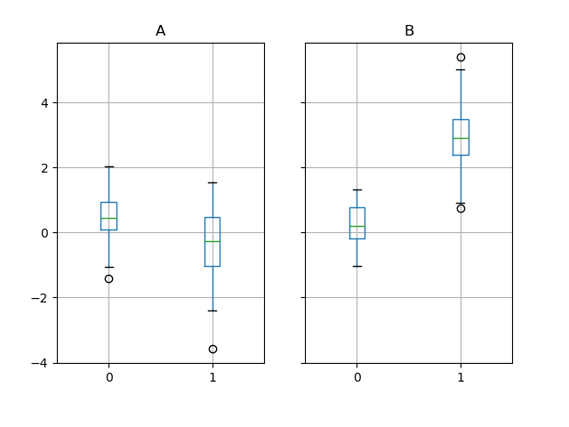
The result of calling boxplot is a dictionary whose keys are the values of our grouping column g (“A” and “B”). The values of the resulting dictionary can be controlled by the return_type keyword of boxplot. See the visualization documentation for more.
Warning
For historical reasons, df.groupby("g").boxplot() is not equivalent to df.boxplot(by="g"). See here for an explanation.
#Piping function calls
New in version 0.21.0.
Similar to the functionality provided by DataFrame and Series, functions that take GroupBy objects can be chained together using a pipe method to allow for a cleaner,more readable syntax. To read about .pipe in general terms, see here
Combining .groupby and .pipe is often useful when you need to reuse GroupBy objects.
As an example, imagine having a DataFrame with columns for stores, products, revenue and quantity sold. We’d like to do a groupwise calculation of prices (i.e. revenue/quantity) per store and per product. We could do this in a multi-step operation, but expressing it in terms of piping can make the code more readable. First we set the data:
In [214]: n = 1000

In [215]: df = pd.DataFrame({'Store': np.random.choice(['Store_1', 'Store_2'], n),
   .....:                    'Product': np.random.choice(['Product_1',
   .....:                                                 'Product_2'], n),
   .....:                    'Revenue': (np.random.random(n) * 50 + 10).round(2),
   .....:                    'Quantity': np.random.randint(1, 10, size=n)})
   .....:

In [216]: df.head(2)
Out[216]:
     Store    Product  Revenue  Quantity
0  Store_2  Product_1    26.12         1
1  Store_2  Product_1    28.86         1
Now, to find prices per store/product, we can simply do:
In [217]: (df.groupby(['Store', 'Product'])
   .....:    .pipe(lambda grp: grp.Revenue.sum() / grp.Quantity.sum())
   .....:    .unstack().round(2))
   .....:
Out[217]:
Product  Product_1  Product_2
Store
Store_1       6.82       7.05
Store_2       6.30       6.64
Piping can also be expressive when you want to deliver a grouped object to some arbitrary function, for example:
In [218]: def mean(groupby):
   .....:     return groupby.mean()
   .....:

In [219]: df.groupby(['Store', 'Product']).pipe(mean)
Out[219]:
                     Revenue  Quantity
Store   Product
Store_1 Product_1  34.622727  5.075758
        Product_2  35.482815  5.029630
Store_2 Product_1  32.972837  5.237589
        Product_2  34.684360  5.224000
where mean takes a GroupBy object and finds the mean of the Revenue and Quantity columns respectively for each Store-Product combination. The mean function can be any function that takes in a GroupBy object; the .pipe will pass the GroupBy object as a parameter into the function you specify.
#Examples
#Regrouping by factor
Regroup columns of a DataFrame according to their sum, and sum the aggregated ones.
In [220]: df = pd.DataFrame({'a': [1, 0, 0], 'b': [0, 1, 0],
   .....:                    'c': [1, 0, 0], 'd': [2, 3, 4]})
   .....:

In [221]: df
Out[221]:
   a  b  c  d
0  1  0  1  2
1  0  1  0  3
2  0  0  0  4

In [222]: df.groupby(df.sum(), axis=1).sum()
Out[222]:
   1  9
0  2  2
1  1  3
2  0  4
#Multi-column factorization
By using ngroup(), we can extract information about the groups in a way similar to factorize()(as described further in the reshaping API) but which applies naturally to multiple columns of mixed type and different sources. This can be useful as an intermediate categorical-like step in processing, when the relationships between the group rows are more important than their content, or as input to an algorithm which only accepts the integer encoding. (For more information about support in pandas for full categorical data, see the Categorical introduction and the API documentation
In [223]: dfg = pd.DataFrame({"A": [1, 1, 2, 3, 2], "B": list("aaaba")})

In [224]: dfg
Out[224]:
   A  B
0  1  a
1  1  a
2  2  a
3  3  b
4  2  a

In [225]: dfg.groupby(["A", "B"]).ngroup()
Out[225]:
0    0
1    0
2    1
3    2
4    1
dtype: int64

In [226]: dfg.groupby(["A", [0, 0, 0, 1, 1]]).ngroup()
Out[226]:
0    0
1    0
2    1
3    3
4    2
dtype: int64
#Groupby by indexer to ‘resample’ data
Resampling produces new hypothetical samples (resamples) from already existing observed data or from a model that generates data. These new samples are similar to the pre-existing samples.
In order to resample to work on indices that are non-datetimelike, the following procedure can be utilized.
In the following examples, df.index // 5 returns a binary array which is used to determine what gets selected for the groupby operation.
Note
The below example shows how we can downsample by consolidation of samples into fewer samples. Here by using df.index // 5, we are aggregating the samples in bins. By applying std() function, we aggregate the information contained in many samples into a small subset of values which is their standard deviation thereby reducing the number of samples.
In [227]: df = pd.DataFrame(np.random.randn(10, 2))

In [228]: df
Out[228]:
          0         1
0 -0.793893  0.321153
1  0.342250  1.618906
2 -0.975807  1.918201
3 -0.810847 -1.405919
4 -1.977759  0.461659
5  0.730057 -1.316938
6 -0.751328  0.528290
7 -0.257759 -1.081009
8  0.505895 -1.701948
9 -1.006349  0.020208

In [229]: df.index // 5
Out[229]: Int64Index([0, 0, 0, 0, 0, 1, 1, 1, 1, 1], dtype='int64')

In [230]: df.groupby(df.index // 5).std()
Out[230]:
          0         1
0  0.823647  1.312912
1  0.760109  0.942941
#Returning a Series to propagate names
Group DataFrame columns, compute a set of metrics and return a named Series. The Series name is used as the name for the column index. This is especially useful in conjunction with reshaping operations such as stacking in which the column index name will be used as the name of the inserted column:
In [231]: df = pd.DataFrame({'a': [0, 0, 0, 0, 1, 1, 1, 1, 2, 2, 2, 2],
   .....:                    'b': [0, 0, 1, 1, 0, 0, 1, 1, 0, 0, 1, 1],
   .....:                    'c': [1, 0, 1, 0, 1, 0, 1, 0, 1, 0, 1, 0],
   .....:                    'd': [0, 0, 0, 1, 0, 0, 0, 1, 0, 0, 0, 1]})
   .....:

In [232]: def compute_metrics(x):
   .....:     result = {'b_sum': x['b'].sum(), 'c_mean': x['c'].mean()}
   .....:     return pd.Series(result, name='metrics')
   .....:

In [233]: result = df.groupby('a').apply(compute_metrics)

In [234]: result
Out[234]:
metrics  b_sum  c_mean
a
0          2.0     0.5
1          2.0     0.5
2          2.0     0.5

In [235]: result.stack()
Out[235]:
a  metrics
0  b_sum      2.0
   c_mean     0.5
1  b_sum      2.0
   c_mean     0.5
2  b_sum      2.0
   c_mean     0.5
dtype: float64


更多建議: